Build your own dithering algorithm
Sweetcorn supports the use of custom dithering algorithms if you want to create your own approach.
Threshold map dithering
Section titled “Threshold map dithering”Understanding threshold maps
Section titled “Understanding threshold maps”A threshold map is a two-dimensional tile of values against which pixels are tested in order to decide if they should be dithered to black or white.
Imagine, for example, a very simple image of 4 pixels by 4 pixels showing a gradient from black in the top left, to a brighter grey in the bottom right.
Each pixel has an intensity between 0 and 255:
0 30 60 90 30 60 90 120 60 90 120 150 90 120 150 180The simplest possible threshold map consists of just a single value. Every pixel in the image will be tested against that same value in order to decide whether to set it to black or white.
For example, if we divided the 0–255 range in half, we could test each pixel in an image against 127.
This is what Sweetcorn’s built-in threshold algorithm does.
Pixels with a value lower than 127 would be set to 0 and pixels with a value higher than 127 would be set to 255.
For our 4×4 example image, the result would look like this:
0 0 0 0 0 0 0 0 0 0 0 255 0 0 255 255A lot of data is lost when using such a simple threshold map.
Even if a pixel’s value is 120, it still ends up set to 0, while a pixel with a value of 130 — only slightly brighter — ends up set to 255.
The average pixel intensity of our original example image was 90, but after applying the threshold, it’s roughly 48, so the image got a lot darker too.
To improve on a single-value threshold, we can create a map that contains multiple values, which we tile over the image. For any given pixel of our image the errors remain, but the errors average out, producing a result that is perceptually closer to the original image.
For example, we could use a 2×2 threshold map containing a range of thresholds:
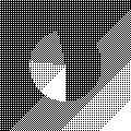
0 128192 64This is the smallest of the classic Bayer threshold maps.
The value at (0, 0) in the threshold map applies to the pixel at (0, 0) in the image, but also to the pixels at (2, 0), (0, 2), and (2, 2), because we tile the threshold map to cover the full image.
If we apply this to our original pixel data we get the following result:
0 0 255 0 0 0 0 255255 0 255 255 0 255 0 255We can see that with this threshold map, some values that were previously set to 0 are now set to 255 and we get a slightly more gradual transition from black in the top left to white in the bottom right.
Here’s an example of a similar image dithered using this matrix:
See “Threshold maps” on the algorithms page for more examples of Sweetcorn’s built-in maps.
Defining a custom threshold map for Sweetcorn
Section titled “Defining a custom threshold map for Sweetcorn”In Sweetcorn, threshold maps are defined as two-dimensional arrays of numbers in the range 0–255.
For example, the 2×2 Bayer map shown above would be defined like this:
const bayer2 = [ [0, 128], [192, 64],];Threshold maps do not have to be square, they can also be rectangular. However, each row in the map must be the same length.
You can provide your custom threshold maps when using sweetcorn() or a framework integration.
When using the Node.js API, pass your threshold map as the thresholdMap option:
await sweetcorn(image, { thresholdMap: bayer2 });When using the Astro integration, provide your custom threshold maps in the options object:
export default { integrations: [ sweetcorn({ customThresholdMaps: { 'my-map:': bayer2, }, }), ],};You can then reference your custom map’s name to use it:
<Image dither="my-map" src={example} alt="Example" />Error diffusion dithering
Section titled “Error diffusion dithering”Understanding error diffusion
Section titled “Understanding error diffusion”Dithering using error diffusion attempts to address the difference between an image’s original pixel values and the quantized black or white result caused by applying a threshold.
When a pixel is quantized to black or white, there is usually some error between the original pixel value and the quantized value.
For example, if a pixel has an original value of 100 and is quantized to 0, the error is 100.
In error diffusion dithering, this error is distributed (“diffused”) to neighbouring pixels that have not yet been processed.
This means that, for example, for an area of pixels all with the value 60, most of these pixels will be rounded down to 0, but eventually the error will build up, pushing one of these pixels past the threshold, so it gets set to 255.
How quantization errors are diffused is determined by a diffusion “kernel”.
Let’s look at an example using a very simple two-dimensional kernel, the same one included in Sweetcorn as simple-diffusion:
* 0.50.5 0This kernel takes the error for the current pixel (indicated by the *) and adds half of it to the pixel to the right, and half of it to the pixel to the left.
Let’s look at an example using an image where all the pixels are 60:
60 60 60 60 60 60 60 60 60 60 60 60We look at the first pixel.
Because it is less than 128, it gets set to 0.
The error of 60 is divided between the pixels below and to the right:
0 90 60 60 90 60 60 60 60 60 60 60We continue this for each pixel in the first row and end up with an image where each pixel in the second row contains an increasing amount of error from the pixel above:
0 0 0 0 90 105 113 116 60 60 60 60When we start processing row two, the error for the first pixel is now 90 and distributed in the same way:
0 0 0 0 0 150 113 116105 60 60 60We now have our first example of the diffused error passing the threshold! The second pixel in row two will be white when processed, and produce a negative error which is deducted from the neighbouring pixels:
0 0 0 0 0 255 61 116105 7 60 60If we continue this process for all pixels we end up with this image:
0 0 0 0 0 255 0 255 0 0 0 0While it’s not very obvious in this small example, the diffusion process helps to represent the shades between black and white by creating areas where the mix of black and white pixels approximates the original shade of grey.
Here’s an example of a test image dithered using this same simple-diffusion kernel:
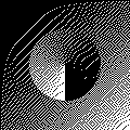
The small size of this simple kernel produces some recognisable artifacts in the form of diagonal lines. Larger kernels, which distribute the error in smaller amounts across more pixels, are more expensive to compute but tend to produce fewer artifacts.
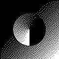
For example, the Atkinson kernel (named for Bill Atkinson who developed it at Apple in the 1980s), distributes ⅛ of the error to 6 different pixels:
0 * 0.125 0.1250.125 0.125 0.125 0 0 0.125 0 0Atkinson dithering produces fewer artifacts and also higher contrast, because only 75% of each pixel’s error is diffused:
See “Error diffusion” on the algorithms page for more examples of Sweetcorn’s built-in kernels.
Defining a custom diffusion kernel for Sweetcorn
Section titled “Defining a custom diffusion kernel for Sweetcorn”In Sweetcorn, diffusion kernels are defined as two-dimensional arrays of numbers in the range 0–1. The middle value in the first row is treated as the current pixel (rounded down for rows of an even length, e.g. for a 4-pixel-wide kernel, the second value in the row is the current pixel, not the third).
For example, the Atkinson diffusion kernel shown above is defined like this:
const atkinson = [ [0, 0, 0.125, 0.125], [0.125, 0.125, 0.125, 0], [0, 0.125, 0, 0],];Each row in the map must be the same length. The value for the current pixel and any preceding pixels in the first row must be 0.
You can provide your custom diffusion kernels when using sweetcorn() or a framework integration.
When using the Node.js API, pass your diffusion kernel in the options object:
await sweetcorn(image, { diffusionKernel: myKernel });When using the Astro integration, provide your custom diffusion kernels via the integration options:
export default { integrations: [ sweetcorn({ customDiffusionKernels: { 'my-kernel': myKernel, }, }), ],};You can then reference your custom kernel’s name to use it:
<Image dither="my-kernel" src={example} alt="Example" />